

A Python Package for Adaptive Spatio-Temporal Exploratory Model (AdaSTEM)


pip install stemflowFor optional memory monitoring (psutil) and tuning (XGBoost and Optuna):
pip install "stemflow[monitoring,tuning]"Use stemflow[monitoring] or stemflow[tuning] to install either separately.
To install the latest version from GitHub:
pip install "stemflow @ git+https://github.com/chenyangkang/stemflow.git"Or using conda:
conda install -c conda-forge stemflowstemflow is a toolkit for Adaptive Spatio-Temporal Exploratory Model (AdaSTEM [1, 2]) in Python. Typical usage is daily abundance estimation using eBird citizen science data (survey data).
stemflow adopts "split-apply-combine" philosophy. It
- Splits input data using Quadtree or Sphere Quadtree.
- Trains each spatiotemporal split (called stixel) separately.
- Aggregates the ensemble to make the prediction.
The framework leverages the "adjacency" information of surroundings in space and time to model/predict the values of target spatiotemporal points. This framework ameliorates the long-distance/long-range prediction problem [3], and has a good spatiotemporal smoothing effect.
For more information, please see an introduction to stemflow and learning curve analysis
Main functionality of stemflow |
Supported indexing | Supported tasks |
|---|---|---|
| ✅ Spatiotemporal modeling & prediction |
✅ User-defined 2D spatial indexing (CRS) |
✅ Binary classification task |
| ✅ Calculate overall feature importances |
✅ 3D spherical indexing |
✅ Regression task |
| ✅ Plot spatiotemporal dynamics |
✅ User-defined temporal indexing |
✅ Hurdle task (two step regression – classify then regress the non-zero part) |
| ✅ Spatial-only modeling |
||
| For details see AdaSTEM Demo | For details and tips see Tips for spatiotemporal indexing | For details and tips see Tips for different tasks |
| Supported data types | Supported base models |
|---|---|
| ✅ Both continuous and categorical features (prefer one-hot encoding) |
✅ sklearn style BaseEstimator classes (you can make your own base model), for example here |
| ✅ Both static (e.g., yearly mean temperature) and dynamic features (e.g., daily temperature) |
✅ sklearn style Maxent model. Example here. |
| For details and tips see Tips for data types | For details see Base model choices |
Use Hurdle model as the base model of AdaSTEMRegressor. This example uses XGBoost, so install the tuning extra shown above:
import numpy as np
from stemflow.model.AdaSTEM import AdaSTEM, AdaSTEMClassifier, AdaSTEMRegressor
from stemflow.model.Hurdle import Hurdle
from xgboost import XGBClassifier, XGBRegressor

## "hurdle in Ada"
model = AdaSTEMRegressor(
    base_model=Hurdle(
        classifier=XGBClassifier(tree_method='hist',random_state=42, verbosity = 0, n_jobs=1),
        regressor=XGBRegressor(tree_method='hist',random_state=42, verbosity = 0, n_jobs=1)
    ),                                      # hurdel model for zero-inflated problem (e.g., count)
    save_gridding_plot = True,
    ensemble_fold=50,                       # data are modeled 50 times, each time with jitter and rotation in Quadtree algo
    min_ensemble_required=30,               # Only points covered by > 30 ensembles will be predicted
    grid_len_upper_threshold=25,            # force splitting if the grid length exceeds 25
    grid_len_lower_threshold=5,             # stop splitting if the grid length fall short 5
    temporal_start=1,                       # The next 4 params define the temporal sliding window
    temporal_end=366,
    temporal_step=20,                       # The window takes steps of 20 DOY (see AdaSTEM demo for details)
    temporal_bin_interval=50,               # Each window will contain data of 50 DOY
    points_lower_threshold=50,              # Only stixels with more than 50 samples are trained and used for prediction
    Spatio1='longitude',                    # The next three params define the name of
    Spatio2='latitude',                     # spatial coordinates shown in the dataframe
    Temporal1='DOY',
    use_temporal_to_train=True,             # In each stixel, whether 'DOY' should be a predictor
    n_jobs=1,
    random_state=42
)
Fitting and prediction methods follow the style of sklearn BaseEstimator class:
## fit
model = model.fit(X_train.reset_index(drop=True), y_train)

## predict
pred = model.predict(X_test)
pred = np.where(pred<0, 0, pred)
eval_metrics = AdaSTEM.eval_STEM_res('hurdle', y_test, pred)
print(eval_metrics)
Where the pred is the mean of the predicted values across ensembles.
See AdaSTEM demo for further functionality.
Besides, stemflow also support lazy loading and database query to reduce memory load during parallel computing.
The execution rewrite adds a Pandas-friendly database helper and optional shared training arrays:
from stemflow.lazyloading import make_training_databases

X_path, y_path = make_training_databases(X_train, y_train, "data/training")
model.fit(X_path, y_path, temporal_window_prequery=True,
          training_data_backend="memmap", inner_max_num_threads=1,
          max_concurrent_ensembles=4)
Native Pandas, DuckDB or Parquet execution remains the default; memory-mapped execution is optional. See the parallel execution guide and executed example for compatibility, scratch-space requirements and complete-job memory trade-offs. The repository also contains reproducible benchmarks in scripts/00_benchmarks/ and measured comparisons in resources/REWRITE.md.
For optional live wall timings and parent/worker memory, install stemflow[monitoring] and wrap fitting and prediction in with model.monitor_execution(output_path="data/execution_monitor.json") as monitor:. The monitor reports sampled process-tree peaks, named stages and optional flushed log updates. Its plain report remains available as model.execution_monitor_ and survives model saving/loading; it retains summaries by default. RSS uses a portable psutil reader, with optional platform-specific USS/PSS/footprint measurements. See the monitoring guide for interpretation and target-machine checks.
Mean predictions now support streaming ensemble aggregation. Optional calibration and tuning wrappers can be used independently or together, inside or outside AdaSTEM. The pipeline report compares timings, peak memory, calibration diagnostics and compatibility limits.
model.gridding_plot
# Here, the model is a AdaSTEM class, not a hurdle class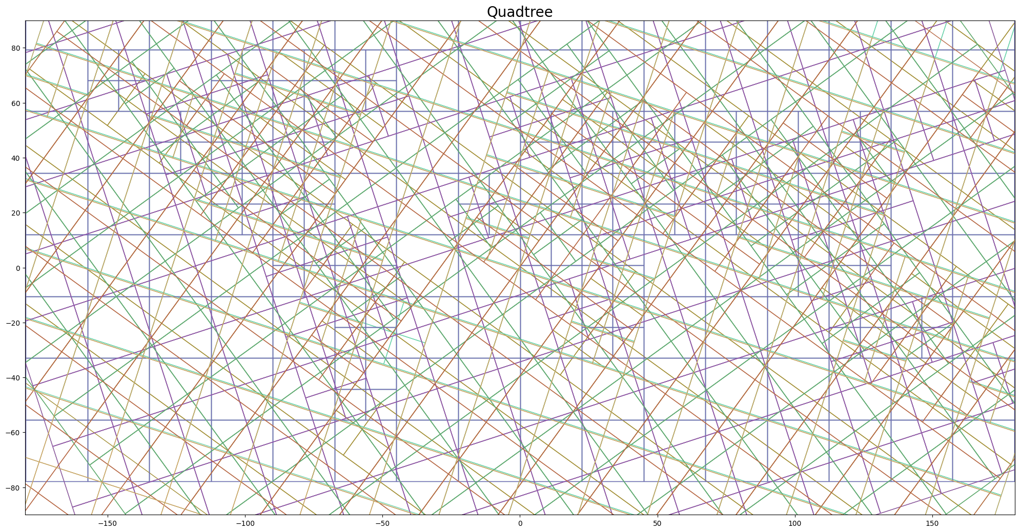
Here, each color shows an ensemble generated during model fitting. In each of the 10 ensembles, regions (in terms of space and time) with more training samples were gridded into finer resolution, while the sparse one remained coarse. Prediction results were aggregated across the ensembles (that is, in this example, data were modeled 10 times).
If you use SphereAdaSTEM module, the gridding plot is a plotly generated interactive object by default:

See SphereAdaSTEM demo and Interactive spherical gridding plot.
Daily Abundance Map of Barn Swallow

See section AdaSTEM demo for how to generate this GIF.
Chen et al., (2024). stemflow: A Python Package for Adaptive Spatio-Temporal Exploratory Model. Journal of Open Source Software, 9(94), 6158, https://doi.org/10.21105/joss.06158
@article{Chen2024,
  doi = {10.21105/joss.06158},
  url = {https://doi.org/10.21105/joss.06158},
  year = {2024},
  publisher = {The Open Journal},
  volume = {9},
  number = {94},
  pages = {6158},
  author = {Yangkang Chen and Zhongru Gu and Xiangjiang Zhan},
  title = {stemflow: A Python Package for Adaptive Spatio-Temporal Exploratory Model},
  journal = {Journal of Open Source Software}
}We welcome pull requests. Contributors should follow contributor guidelines.
Application-level cooperation is also welcomed. We recognized that stemflow may consume large computational resources especially as data volume boosts in the future. We always welcome research collaboration of all kinds.
References: