Deepwave

Upgrading from v0.0.27? Deepwave 0.1.0 has breaking interface changes. The upgrading guide explains the changes and replacements, including output tuple indices that can change meaning without raising an error.

Deepwave provides wave propagation modules for PyTorch, for applications such as seismic imaging and inversion. It performs forward modelling and backpropagation, so it can simulate wave propagation to generate synthetic data, or invert for the scattering potential (reverse-time migration, RTM, or its least-squares counterpart, LSRTM), other model parameters (full-waveform inversion, FWI), initial wavefields, or source wavelets. It can also be used inside a larger chain of operations, with forward and backpropagation flowing through the whole chain end to end. You can use your own objective functions, or functions that generate the propagator's inputs, and PyTorch's automatic differentiation calculates how to backpropagate through them. New to seismic/wave-equation terminology? The glossary defines the terms (PML, CFL, Born, FWI, and more) used throughout this README and the rest of the documentation.

Deepwave requires Python 3.9 or later and PyTorch 2.4 or later. First install PyTorch for your CPU or CUDA device using the instructions on the PyTorch website. Then install Deepwave:

    pip install deepwave

macOS wheels support Apple Silicon. Intel Mac wheels are no longer provided: PyTorch 2.4 and newer do not publish wheels for that platform.

Prebuilt x86 wheels require AVX2. Older CPUs need a source build; see installation troubleshooting.

PyTorch is Deepwave's only dependency. The example scripts under docs/ additionally import matplotlib (to draw their figures) and, in some cases, numpy, scipy (smoothing and filter design), torchaudio (applying those filters), torchvision and geomloss, but those are needed only to run the examples, never by Deepwave itself. To install all of them:

    pip install 'deepwave[examples]'

The documentation contains examples and instructions on how to install and use Deepwave. You might also like to watch a video summary of Deepwave. Not every propagator supports every option (dimensionality, backend, boundary faces, batching, second-order differentiation, callbacks, ...). See the capability matrix (declared in the code and checked by conformance tests) before assuming a combination works.

Why Deepwave

• Computationally efficient. Deepwave's compiled kernels use a hand-derived adjoint for better performance and lower memory requirements than pure PyTorch implementations. See what Deepwave calculates.
• Second derivatives are supported, not just first. The scalar, acoustic, and elastic propagators can compute Hessian-vector products (derivatives of gradients); see the Hessian example.
• Born (linearised) modelling. Model scattered waves from perturbations to a background medium for linearised inversion and imaging. See the torch.func example.
• Deepwave fits into an ordinary PyTorch workflow. Because propagation is a normal PyTorch autograd Function, it works directly with PyTorch optimisers, DistributedDataParallel over shots, torch.func transforms, and any PyTorch loss function or neural-network model of the input parameters. See the capability matrix for exactly what each propagator supports.

Deepwave does not try to be a general symbolic PDE solver, a multi-node HPC code, or a non-differentiable simulation toolkit — see Devito, SPECFEM, and k-Wave respectively for those needs. If you are choosing between wave-propagation packages, see the comparison guide.

(Note: the DeepWave-KAUST GitHub organisation, home of the SWEEP package, is unrelated to this project.)

Features

• Supports the 1D, 2D, and 3D constant density acoustic / scalar wave equation (regular and Born modelling), variable density acoustic, elastic, viscoacoustic (single-mechanism SLS attenuation), elastic VTI (anisotropic), and pseudo-acoustic VTI (deepwave.acoustic_vti, the Duveneck et al. 2008 V_S=0 reduction) wave equations
• Runs on CPUs and appropriate GPUs
• The gradient of all outputs (final wavefields and receiver data) can be calculated with respect to the model parameters (wavespeed, scattering potential, etc.), initial wavefields, and source amplitudes
• Distributed acoustic sensing (DAS) strain-rate receivers (deepwave.das, including gauge averaging and helically wound fibre response) and transducer-array helpers for ultrasound/NDT (deepwave.transducers)
• Segmented gradient checkpointing (deepwave.checkpointing.run_segments, composed with torch.utils.checkpoint) to bound backward-pass memory for long simulations
• A time-dispersion correction (deepwave.time_dispersion) to remove the leapfrog time-stepping error when running near the CFL limit

Quick Example

This example also needs Matplotlib: python -m pip install matplotlib. On Python 3.9, also install "pyparsing<3.3" for compatibility with Matplotlib 3.9: python -m pip install "pyparsing<3.3". Newer Python versions can use the current Matplotlib and Pyparsing releases.

In a few lines you can make a velocity model, propagate a wave from a source in the top left corner to a receiver in the top right, calculate an objective function, and backpropagate to obtain its gradient with respect to the velocity.

import torch
import deepwave
import matplotlib.pyplot as plt

v = 1500 * torch.ones(100, 100)
v[50:] = 2000
v.requires_grad_()

out = deepwave.scalar(
    v, grid_spacing=4, dt=0.004,
    source_amplitudes=deepwave.wavelets.ricker(25, 200, 0.004, 0.06).reshape(1, 1, -1),
    source_locations=torch.tensor([[[0, 0]]]),
    receiver_locations=torch.tensor([[[0, 99]]]),
    pml_freq=25,
    max_vel=2000,
)

(out.receiver_amplitudes**2).sum().backward()

_, ax = plt.subplots(1, 3, figsize=(9, 3))
ax[0].imshow(v.detach())
ax[0].set_title("Velocity model")
ax[1].plot(out.receiver_amplitudes.detach().flatten())
ax[1].set_title("Receiver data")
ax[2].imshow(v.grad.detach(), vmin=-1e-5, vmax=1e-5)
ax[2].set_title("Gradient")
plt.show()

This objective measures receiver energy; an inversion instead compares predicted data with observations. max_vel and pml_freq fix the numerical setup. At this dt, CFL substepping makes the default model gradient a sampled approximation. For exact discrete model derivatives and finite-difference checks, see the gradient conditions.

(plt.show() only opens a window if a display is available. On a headless machine it does nothing and the script exits without complaint; replace it with plt.savefig("quick_example.png") to see the result in that case.)

(This example never moves anything to a GPU, so it runs on the CPU even if one is available; move v and the other tensors to a GPU with .to(device) to use it, as the quick start guide and the FWI example do.)

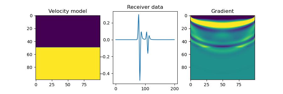
For a line-by-line walkthrough of this same example -- including what pml_freq and the other arguments mean -- see the quick start guide. There are more examples in the documentation.

Example notebooks

A few of the examples are also available as Jupyter notebooks (paired with their .py source via jupytext, so the two stay in sync -- see CONTRIBUTING.md) that you can run directly in Google Colab, no local install required (the first cell installs Deepwave):

Example	Colab
Generated model (quickstart-style FWI)
Elastic FWI
Photoacoustic reconstruction
FWI recipes (OT, soft-DTW, deep image prior, UQ)

Citing

If you would like to cite Deepwave, I suggest:

@software{richardson_alan_2026,
  author       = {Richardson, Alan},
  title        = {Deepwave},
  year         = 2026,
  publisher    = {Zenodo},
  version      = {0.1.0},
  doi          = {10.5281/zenodo.3829886},
  url          = {https://doi.org/10.5281/zenodo.3829886}
}